
What is Airbnb Occupancy Rate
In the hospitality industry the occupancy rate is defined as the number of nights booked over nights available. It is a key metric all Airbnb hosts need to understand to be successful. In this analysis we’ll explore the most important factors driving the Airbnb occupancy rate.
Introduction to the analysis
This analysis looks at a case study of listings in New York City over two years to uncover the factors behind the occupancy rate. Data was sourced from Inside Airbnb, an activist project with the objective to provide data that quantifies the impact of short-term rentals on housing and residential communities. Listing data ranged from January 2018 to February 2020. Importantly, this time extends right up to when COVID-19 measures took effect and before New York instituted it’s 30-day minimum occupancy on short-term rentals.
For this analysis I also pulled in data from Walk Score, a company whose mission is to promote walkable neighborhoods. Walk Score acts as a good approximation of proximity of a listing to common amenities such as grocery stores, restaurants, and retail.
As always, my aim is to present this analysis in layman’s terms and focus on the insights. If interested, the full code can be found on the GitHub for this project.
Preparing the data
The Airbnb occupancy rate is a difficult metric to predict. As such, there was a lot of preparation and massaging done to the data.
Defining the occupancy rate
This analysis uses publicly available data. We’ll be using the host’s public-facing calendars to infer the number of days booked. By using these calendars, we have no way of knowing if a day is unavailable because it is booked or because the host did not make it available. In other words, we are dealing with incomplete information and because of this we’ll need to make a lot of assumptions.
To handle this, I first excluded listings with either 0 days available or 30 days available. If a listing had 0 days available, I’m broadly assuming that the host didn’t make those days available to book. If a listing had 30 days available I’m broadly assuming that the host is not actively managing the calendar.
Of course, by doing this I ended up dropping some false positives from the data set. That is, listings legitimately fully booked over 30 days or had 0 bookings. But I assumed by taking this step I was losing more bad data than good data.
Next, I wanted to ensure that the dataset only featured actively managed listings. To do this, I removed listings with calendars not updated in over 2 months and had less than three reviews.
Finally I created the occupancy variable by subtracting the number of available days in the calendar in the next 30 from 30. This gave me an approximation of number of days booked (occupancy) over the next 30 days.
Constraining the dataset
After creating the occupancy variable, I had to define the dataset I would use to predict it. I started by considering that the occupancy rate is really another way of saying “how much available business did a listing earn?” So, to be fair, the dataset should be constrained to only listings that are competing for the same business.
However, if I were to truly accomplish this every listing would need to accommodate the same number of guests, have the same minimum nights, etc. The universe of data would become too small to model.
I decided a compromise would be to constrain the dataset to listings that accommodate four or fewer guests and had three of fewer minimum nights.
Other data massaging
Even though I constrained listings to those that could accommodate four or fewer guests, there is still a huge difference in the price for listings that accommodate one guest and those that accommodate four. Therefore, to normalize price, I created a metric called “price per accommodates” that is the nightly rate divided by the number of guests accommodated.
I also decided that because there are so many assumptions being made about the variable we’re trying to predict (occupancy rate) it didn’t make sense to try to predict the exact number. Rather, it would make more sense to predict within a range of occupancy rates. For these ranges, I defined low occupancy as 1-10 days booked in the next 30 days. Medium occupancy was 11-19 days booked in the next 30 days and high occupancy was 20+ days booked in the next 30 days.
The last step in preparing the data for modeling was to one-hot-encode the categorical variables and normalize the numeric variables. The final list of features used in the model is as follows.
Features used in model
- Price per accommodates: nightly rate divided by guests accommodated
- Room type: entire place, shared room, or private room
- Superhost status
- Host total listings count: number of listings under management by the same host
- Security deposit
- Cleaning fee
- Extra guest fee
- Instant Bookable: the listing has Instant Book enabled or not
- Cancellation policy: flexible, moderate, or strict
- Month: month of the host’s calendar
- Listings per square km: listings in the neighborhood divided by area of the neighborhood in kilometers
- Walk Score: how walkable the neighborhood is in terms of proximity to amenities such as grocery stores, restaurants and retail. Measured on a scale of 1 to 100.
- Property type: House, apartment or other (other is a catchall including condo, townhouse, etc.)
- All category ratings: including value, cleanliness, accuracy, check-in, communication, and location
- The overall rating
- Amenities: excluding amenities that appeared in less than 500 listings in the dataset.
Choosing the model

Because I bucketed the variable I’m trying to predict, I needed a model that would classify the prediction into those buckets. After trying a few different models, I settled on using a gradient boosting classifier to model the data as it’s quite powerful.
However, in machine learning there is generally a trade off between interpretability and predictive power. More simple models can be easier to interpret but may not be as predictive as more complex models. More complex models which rely on complicated algorithms are often called black boxes. They can give you a more accurate prediction, but explaining how the model made that prediction can be more challenging.
How the model works
To explain in the simplest terms what’s happening in a gradient boosting model first imagine a decision tree for a single listing. With this decision tree, we’re trying to predict occupancy rate using every feature we have for that listing. As we move from the top of the tree to the bottom, each feature will help decide if we expect that listing to have low, medium, or high occupancy.
Recall that we also know the actual occupancy of this listing. So when we get to the bottom of the tree we’ll know if the prediction was correct or not.
Now imagine doing this for every single listing. We would start to get an idea of which features were useful in making an accurate occupancy rate prediction and which were not. Then, we could improve the predictive power by throwing out the bad trees that weren’t good at making predictions and keep the good ones. We could also continue to build new trees off what we learned from the good trees. That is essentially what is happening in a gradient boost model.
The resulting model correctly predicted the occupancy 58% of the time.
Interpreting the model
One approach to interpreting the output of the gradient boost model (or any “black box” algorithmic type model for that matter) is to use Shapley values.
The Shapley value is a concept that comes from game theory. In very simple terms, it assigns a value for how much each individual “actor” contributed to an outcome.
For our purposes, it will tell us how much each individual feature modeled contributed to the prediction of occupancy (low, medium, or high). If we then take the average of the absolute value of Shapley values from every single prediction the model made, we’ll see which features were most important.
The following plot shows this with each color showing how important a feature was to that predicted level of occupancy.
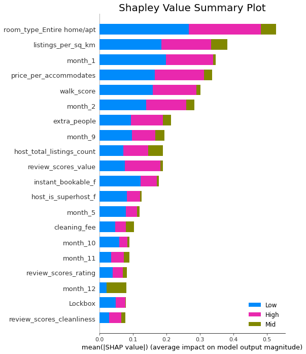
Most important Airbnb occupancy rate factors ranked
From this plot we can see not only which factors are important to the Airbnb occupancy rate, but we can rank them from most important to less important.
- Listing the entire place
- Competition
- Seasonality
- Price
- Proximity to amenities
- Listings under management
- Extra guest fee
- Value score
- Instant bookable
- Superhost status
The previous plot only showed us the average absolute Shapley values for each feature. To understand which direction the feature moves a prediction, we’ll need a different view.
Examining an individual prediction
First let’s consider a single data point for which the model predicted high occupancy. The chart below tells us which direction each feature of this listing moved the prediction. The red bars had a positive impact on the prediction and the blue bars a negative impact.
Recall that categorical variables were one-hot encoded so 1 indicates the feature was present and 0 indicates it was absent. Numeric values were normalized so positive values indicates the value of the feature was above average (whereas a negative value indicates below average).
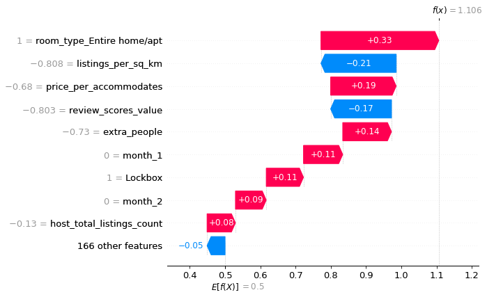
In this plot, we see the feature having the greatest influence on the prediction is room_type_Entire home/apt = 1. In other words, this listing was an entire home and not a shared room or private room. This contributed positively to the prediction of high occupancy.
Next we see listings_per_sq_km is -0.808 indicating this listing was in a neighborhood with lower than average competition. This pushed the prediction away from high occupancy.
As we continue down the plot we see the listing has a below average price. This contributed positively to the high occupancy prediction. It also had a lower than average value rating which contributed negatively.
Ultimately, the push and pull of these features resulted in the prediction of high occupancy.
Examining all predictions
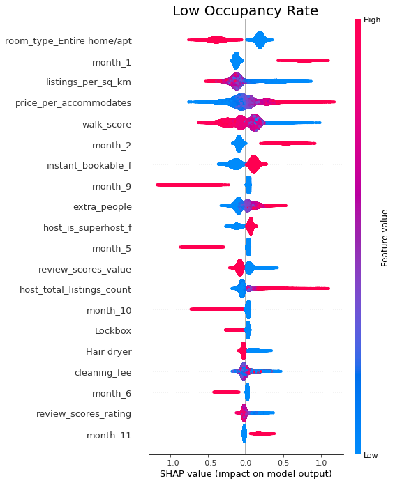
Now we’ll take this same approach for every single prediction of a given outcome. In these plots, blue values indicate low feature values and red indicates high feature values. Points residing to the right of the line had a positive contribution to making a prediction and to the left a negative.
This first plot shows the features used to predict low occupancy.
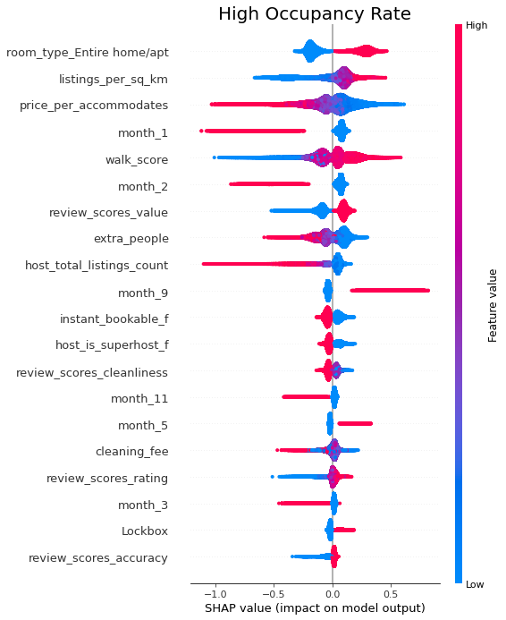
This next plot shows the features used to predict high occupancy.
Defining the factors that determine Airbnb occupancy rate
The above plots give us more context about the factors that have the greatest influence on the occupancy rate. While a lot of it is intuitive, it’s helpful to see it proven out mathematically.
Listing the entire place
Listings that offer the entire space for the guest rather than a private room or a shared room is the most important factor in determining the occupancy rate on Airbnb. Perhaps this is not surprising. It’s the value proposition on which Vrbo has based on a entire recent advertising campaign to differentiate itself from Airbnb. In doing so, they are demonstrating how important this feature is to short-term rental guests.
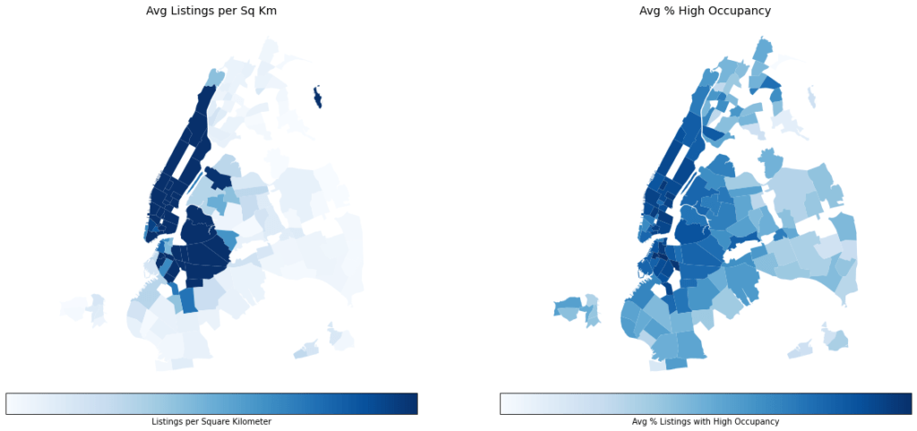
Competition
Competition is the second most important feature in determining the occupancy rate which perhaps is a little counterintuitive. On the one hand we would expect more competition would make it harder to book guests and thus have a negative impact on occupancy. But there is a reason these areas are dense with Airbnb listings – they are popular locations for guests.
Thus, while there may be more competition there are also more guests looking for accommodations. The result is a net positive influence on the occupancy rate. We can see this in the two maps below.
The map on the left shows listings per square kilometer where the dark blue neighborhoods have at least 200 listings per square kilometer. The map on the right shows the average proportion of listings with high occupancy over the entire dataset. At a glance, we can see neighborhoods with more listings also have a higher occupancy rate.
Seasonality
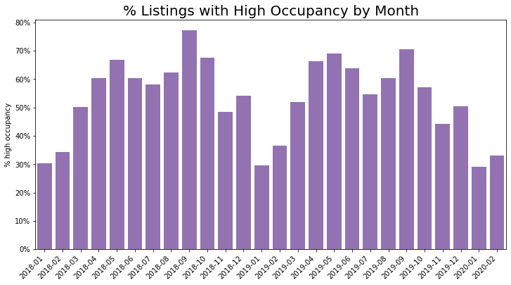
The month of the year appeared multiple times near the top of the Shapley value analysis as a feature determining the occupancy rate. Taking them all together we can say that seasonality is the third most important factor driving the occupancy rate.
In the model, listings from January and February predicted low occupancy. This is not surprising as these are the winter months in New York when we would expect tourism to be at its lowest. It’s not much a stretch to extend this line of thinking to any location where some seasons are busier than others.
In the chart below, we can see % of listings with high occupancy by month dipping in the winter months
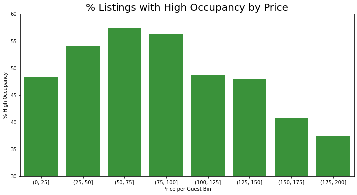
Price
The next most important feature for predicting the occupancy rate is price. A higher price per guest tended to predict lower occupancy whereas a lower price per guest predicted higher occupancy.
In the following chart, listings have been group by price per guest and the average % of listings with high occupancy was calculated. We can see that as price per guest exceeds $100 the % of listings with high occupancy begins to decline.
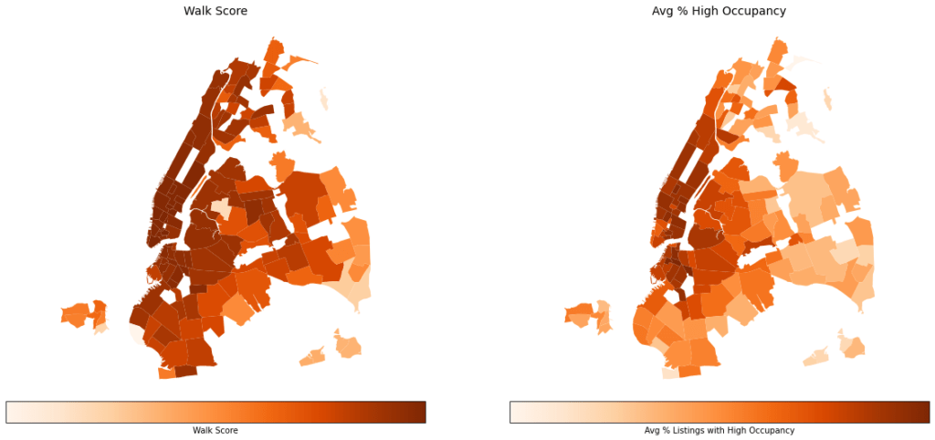
Proximity to amenities
Walk score is a useful stand-in for the overall quality of the location. The score reflects how close a location is to amenities such as restaurants, grocery stores and retail. Higher Walk Scores were a predictor for high occupancy where as lower Walk Scores predicted low occupancy. This shows how important the quality of a location is to the occupancy rate.
We can see this in the maps below. The map on the left shows Walk Score where neighborhoods with higher Walk Scores are colored darker. On the right is the average proportion of listings with high occupancy. At a glance we can see the relationship.
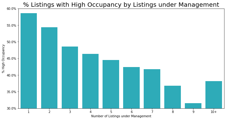
Listings under management
In this model the number of listings under management was a predictor of occupancy where the more listings a host had under management, the lower the predicted occupancy rate was. Interestingly, this is the not first piece of analysis to draw this conclusion.
In a separate analysis on the different segments of hosts using the platform, I estimated that hosts with fewer listings tended to have higher occupancy than management companies with many listings.
We can only speculate as to the reason for this. One explanation would be hosts or companies with many listings are more likely to use pricing or channel management tools. If they are using pricing tools, they could be maximizing their profit through higher pricing and lower bookings. Or it could be that using a channel management tool the listings is being booked across multiple platforms giving the appearance of a lower occupancy rate on Airbnb.
The chart below shows the average proportion of listings with high occupancy by number of listings under management. We can see as number of listings under management rises, the average proportion of listings with high occupancy falls.
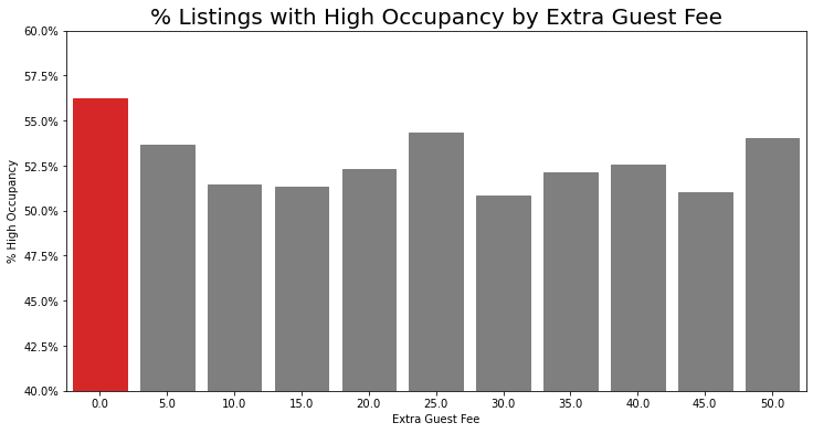
Extra Guest Fee
To understand how the extra guest fee is impacting the occupancy rate, we can look at the graph below. It shows for extra guest fees in $5 increments starting from $0 the average % of listings with high occupancy in the dataset. For $0 the % occupancy is noticeably higher than all other fees. This agrees with the output of the Shapley value analysis. We can generalize and say that having no extra guest fee contributes positively to a higher occupancy rate.
Value Score
Value was the only category rating that appeared in the top 10 ranked factors driving occupancy. We also know that value is one of the most important categories the guest considers when deciding the overall rating. Given that value is so important in the occupancy rate goes to show why it’s important for hosts to understand how Airbnb guests define value.
Instant Book
Interestingly, this feature was a strong predictor of low occupancy but less so for medium and high occupancy. What this tells us is that having Instant Book enabled is more of a difference maker for hosts experiencing low occupancy than those with high occupancy. This makes sense as hosts with high occupancy are unlikely to be gaining from whatever benefit enabling Instant Book provides whereas for hosts with a low occupancy rate it might be worthwhile to enable.
As to why enabling Instant Book would help listings with low occupancy, there are two ways to look at it. On the one hand, it could be that Instant Book makes it easier for guests to book a listing thus increasing the occupancy rate. On the other hand, it’s commonly believed that having Instant Book enabled helps with Airbnb SEO. Either way it is something to consider for hosts with a low occupancy rate.
Superhost Status
We can interpret the impact of Superhost status on the occupancy rate similarly to how we viewed Instant Book. On the one hand, it’s earned by maintaining a high overall rating and having a high response rate. Both of which have a positive influence on the occupancy rate. On the other hand, much like Instant Book, Superhost status is viewed as a positive contributor to Airbnb SEO. Both reasons support why having Superhost status has a positive influence on occupancy rate.
Interpreting factors driving the Airbnb occupancy rate
While all the factors identified above influence the occupancy rate, there is even greater value in being able to interpret these factors.
Understanding which factors are more important than others can allow hosts to prioritize their efforts. For example, a host looking to improve their occupancy rate can turn on Instant Book. But doing so would not have as much of an effect on improving the occupancy rate as optimizing pricing.
Hosts can also derive value from this analysis by understanding which factors are within their control and which are not. From there, a host can focus on improving factors within their control (such as the value rating) while planning for factors outside of their control (such as seasonality).
So far in this write-up we’ve focused on the top 10 factors driving occupancy. However, factors outside the top 10 can also how have impact on the occupancy rate to a lesser extent.
Does the cleaning fee affect the Airbnb occupancy rate
One such feature that has a lesser but not insignificant impact on the occupancy rate is the cleaning fee. As one could imagine, higher cleaning fees predict a lower occupancy rate and lower cleaning fees predict a higher occupancy rate. This would be another area for hosts to examine if they wanted to improve their occupancy rate.
Does the overall rating affect the Airbnb occupancy rate
Likewise, the overall rating appeared just outside the top 10 factors identified in this analysis. Higher overall ratings predicted a high occupancy rate. Hosts looking to improve their occupancy rate should therefore try to improve their overall rating. To do so, hosts should look at the cleanliness of their listing, the accuracy of their description and the value they create. These are the things guests consider most when deciding the overall rating.
Other features with minimal influence on occupancy rate
The type of place (house/apartment/other) did not have a significant influence on the predicted occupancy rate. The type of cancellation policy the host had did not either. This indicates guests are not discriminating on the strictness of the cancellation policy. The amount of the security deposit did not appear to have a strong influence on the occupancy rate. Finally, outside of the value rating, other individual category ratings had minimal influence on the occupancy rate.
Individual amenities mostly do not affect the occupancy rate
Other than lock box appearing in the Shapley value analysis, amenities weren’t a significant driver in predicting the occupancy rate. Meaning, for the most part adding amenities to a listing does not influence occupancy directly.
Of course there are hosts with anecdotal evidence that adding a pool or a hot tub increased their occupancy rate which could certainly be true. However, this model suggests that in general there are more important factors driving the occupancy rate.
Having said that, we know that amenities play a part in creating value. Thus, adding amenities which increase the value of a listing can increase occupancy indirectly.
Limitations of the model
As with the pricing model, any occupancy rate model that uses Airbnb data but does not consider the motivations of hosts will be limited. In the host segmentation analysis, we uncovered the part-time selective and part-time passive hosts, both of which have lower acceptance rates. For these types of hosts we can assume the lower acceptance rate and their decision to host part time make their goals different from full-time hosts. More complex models would need to consider these goals to more accurately predict the occupancy rate.
Key Takeaways
- In this analysis we ranked the top ten factors influencing Airbnb occupancy rate which are:
- Listing the entire place
- Competition
- Seasonality
- Price
- Proximity to amenities
- Listings under management
- Extra guest fee
- Value rating
- Instant Book
- Superhost status
- Features ranked higher are more likely to influence the occupancy rate than lower ranked features
- Hosts should consider what is within their control and what is outside of their control. Optimize what is within your control and plan for what is outside your control.